n,k Characterization

n,k Characterization works out the optical constants of one film on a known substrate from a measurement of it. Feed it reflectance and transmittance from a spectrophotometer, or a Ψ and Δ pair from an ellipsometer. The thickness can be held at a value you already know, or fitted along with the constants.

What comes out is a material you can save and use in designs. It describes the film your process deposits, which is not the same thing as a handbook material with the same chemical name.

What n and k are

The refractive index is complex, n + ik. Both parts change with wavelength and neither has units.

	What it does	How to read it
n, refractive index	Sets the phase the light picks up crossing the film. With the thickness, it sets where the interference fringes fall.	Dielectric coating materials sit between about 1.35 and 2.6. A metal can have n well below 1, and that is real, not an error.
k, extinction coefficient	Sets how fast the light is absorbed inside the film.	k = 0 is a film the model treats as transparent. Bigger k absorbs harder at that wavelength.

k is not the fraction of light the sample absorbs. Inside the material the intensity falls as exp(-4πkz/λ), for a distance z travelled and a wavelength λ in the same units. What the sample actually absorbs also depends on reflection and interference.

Setting up an R/T measurement

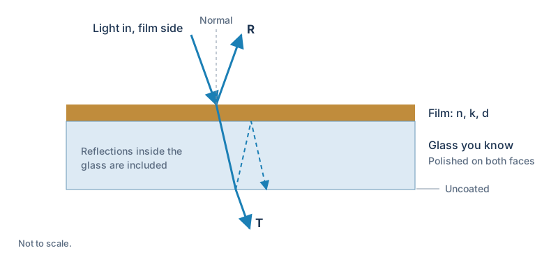
Coat one face of a substrate you know, polished on both faces, and leave the other face bare. A coated glass witness is the usual thing. This is the only sample the window models: the rear face is part of the calculation rather than a nuisance to be removed, and there is no setting that takes it out.

The calculation covers the film, the path through the glass, and the reflection off the bare rear face, combining the repeated passes through the glass as intensities.

The window models one film. A second coating, an adhesion layer thick enough to matter optically, or a sample that scatters, needs more than it can describe.

Measure absolute R and T over wavelengths that overlap. T has to be the light coming out of the whole sample, glass included. A ratio against bare glass, an optical density, or data with the rear-face loss already taken out are not the T this expects. If your instrument writes percentages, confirm the scale when you import.

Import the curves in Measured Spectra, pick T / R, and choose both. In Settings, set the substrate material and its thickness.

Checking the window against a design you already have

A good way to see what this window does is to feed it a spectrum you generated yourself: build the film as a design, export its spectrum, import that back, and characterize it. The film should come back.

Export it with the whole-slab evaluation, not FRONT or BACK. A FRONT export is the coated surface on its own, with no substrate rear face, which is not something an instrument can measure and not what this window fits. Feeding one in reports “These curves are of the coated surface alone” and stops, because the rear face is worth about four percentage points of reflectance on glass and the two do not invert to the same film.

Measuring at an angle

Each curve carries its own angle and polarization, and the fit uses them. The angle is from the normal, so 0° is straight on. T at 0° and R at 8° fit together; the two do not have to match.

Check these on the curve cards in Measured Spectra. They describe the measurement, not the design that happens to be open, and a curve imported without an angle arrives as 0°. Off normal, set the real s, p or average polarization, where average is an equal mix of the two intensities.

The coated face is toward the beam. That is how a witness is measured, and the model has no other orientation.

If the back face is not polished

Polish both faces. The window models one sample, a film on a substrate polished on both sides, and there is no setting that changes it. A witness is cheap and this is what it is for.

If you have to measure a ground-back sample anyway, the useful thing to know is that grinding scatters light, it does not absorb it. Total R and T are close to what a polished witness gives; what a ground face destroys is the specular beam. So measure it on an integrating sphere in total mode, and the calculation still describes it. A straight-through detector loses most of the transmitted beam and that T is not a measurement of anything.

What it does cost you is the light that leaves and never comes back, scattered outside the sphere port or trapped inside the glass. That missing light is indistinguishable from absorption in your film. Losing one percent of T makes a transparent film come back with k of roughly (fraction lost) x λ/(4πd), which is 9e-4 for a 500 nm film at 550 nm, ten times the smallest k that measurement can resolve. It shows up as k rising toward longer wavelengths and the rising-k notice fires. n and thickness survive a ground back; k does not.

A small wedge, which is the usual kind, deviates the transmitted beam by well under a degree and changes T not at all.

If your rear reflection really has been removed, by black glass contacted with matching fluid or the like, this window cannot fit that measurement: the rear face is worth about four percentage points of reflectance on bare glass, forty times photometric accuracy. It will say so with a large residual or refuse to invert, rather than quietly hand you the wrong film.

The model assumes you collect the light the rear face sends back. A stop or an accessory that throws some of it away changes measured R and T in a way this sample model does not know about.

Setting up an ellipsometric measurement

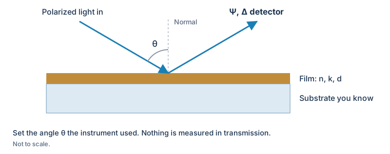
An ellipsometer reads how reflection changes the polarization. Ψ compares the reflected amplitudes of p and s, Δ is the phase between them. Between them they pin down n and k without needing any transmitted light.

Import the pair in Measured Ellipsometry, pick Ψ / Δ, and choose both curves. Check the angle on both, and set the Δ convention in Settings, because the wrong one changes what Δ means. Ψ and Δ at normal incidence say nothing about a coating, and the window refuses them.

The model is one uniform film on a known substrate, read from the coated side, and it assumes no light comes back off the rear face. Clear glass sends rear reflections into the detector whether or not the instrument is an ellipsometer, so use whatever your instrument provides for killing them. Mixed rear reflections, depolarized data, a roughness layer and extra surface layers are all outside what this models.

How thick the film has to be

A film only tells you its index if the measurement can see it. Below roughly a quarter wave of optical thickness at the middle of your range there is little for the fit to read, and a film whose index sits close to the substrate’s leaves even less.

Measured on BK7, with the thickness fitted rather than held:

Film	n	Thinnest that R/T recovers	Thinnest that Ψ/Δ recovers
MgF2	1.38	160 nm	60 nm
SiO2	1.46	100 nm	130 nm
Ta2O5	2.10	80 nm	100 nm
TiO2	2.45	80 nm	60 nm

Two things to take from it. Ellipsometry reaches thinner films than R/T does, which is the usual reason to reach for it. And a low-index film on glass is the hard case: MgF2 on BK7 barely changes R at all, so R/T needs it half again as thick as the quarter wave before the answer settles.

Under those thicknesses the fit still returns a spectrum that matches the measurement, because more than one film reproduces it. Holding the thickness does not rescue it either: with the film treated as transparent, R passes through a minimum at n = √n_substrate, and an index either side of that minimum gives the same R. Read the notices and the residual, and take a thin film to an ellipsometer.

Picking the model and the thickness

Setting	When to use it
Cauchy	A dielectric over a range where it does not absorb. Start here for any oxide or fluoride.
Sellmeier	Try it when Cauchy leaves a shape in the residual. It is a resonance form rather than a polynomial, so it suits a film whose dispersion really is set by one absorption band out of the range. It is the riskier of the two: on a high-index oxide measured by R/T it can settle on the wrong index and still look smooth.
Drude-Lorentz (metal)	Every metal. It covers the free electrons and any absorption sitting on top of them, and reads the number of oscillators off your data. Gold across the visible needs several; aluminium needs none, and then the Model row says Drude, because that is what it has fitted.
λ range	The part both curves cover and you trust, inside the range your substrate data and your model are good for.

Pick the model for the material and for the range you measured. A smooth curve and a run that finished are not evidence the model fits. Look at Fit and Residual before you save anything.

If a fit will not settle, change the model before you change anything else. The wrong one does not always leave an obvious residual: it can land on a plausible index a long way from the film.

One trap when you are trying models against a spectrum TFStudio itself exported. Several built-in materials are dispersion formulas rather than measured tables: SiO2 is Malitson, MgF2 is Dodge, BK7 is Schott, and all three are Sellmeier. Fit a spectrum built from one of those with Sellmeier and it comes back exact, because you are fitting the formula to itself. That tells you nothing about which model suits a real film. Judge models on a real measurement.

Film → Hold pins the thickness you typed and fits only n and k. Use it when you have measured the thickness some other way.

Film → Solve fits the thickness too. Interference fringes in T give it a starting thickness and a range around it; without them, the value you type sets a range from half to one and a half times it, and the fit stays inside that. So the number you type has to be right to about a third. For an opaque metal, hold the thickness: a thick metal film reflects the same however much more you add, and a thickness kept automatically is labelled as assumed rather than measured.

Then press Extract. A run takes from a second to a minute, longest for a metal with the thickness solved on a fine grid. While it works, the control row says which stage it is at and how long it has been running, and Stop ends it.

The three tabs

n and k

Wavelength across the bottom, n on the left axis and k on the right. The k curve and its axis disappear when absorption is below what the measurement could resolve.

• The lines are the smooth dispersion model. This is what Save as material writes.
• The points are separate n and k solved at one wavelength at a time, with the thickness held at the fitted value. Only the ones that solved are drawn. They come out of the same measurement, not out of a second one.

Points sitting on the lines say the model suits the film. Points that drift off it in a pattern say it does not. Points missing or scattered mean the measurement was weak there, noisy, or hard to solve.

The points start from the fitted model, so they can end up on the same branch it did. Agreement between them is a consistency check, not proof the answer is unique or the sample model right.

Fit

Your measured curves and the curves calculated from the fitted model, on top of each other. R and T are drawn as percentages. For ellipsometry Ψ is on the left axis and Δ on the right, both in degrees.

Look at both channels across the whole range. T matching while R misses, or Ψ matching while Δ misses, is not a fit. The wrong substrate, thickness, angle, polarization, Δ convention or model all show up here.

Residual

Calculated minus measured, against wavelength. Zero is agreement, positive means the calculation came out high.

For R and T this is in percentage points: calculated 90.2% against measured 90.0% is +0.2, not a 0.2% relative error. For Ψ and Δ it is degrees, and Δ takes the short way round the circle, so 359° and 1° are 2° apart, not 358°.

What you want is small and shapeless, about the size of your measurement error. A steady offset, a repeating wobble, or a bump in one place is a systematic problem. The shape narrows down what to look at without naming it. This tab is where a mismatch shows when the two curves on Fit look identical.

Reading the results table

The table gives RMS and max for each channel. R and T are fractions here, unlike the percentage points on the chart, so an RMS of 1e-3 is a tenth of a percentage point. Ψ and Δ are degrees in both places.

Photometry raises a notice when the RMS passes 0.003 in R or T, which is three times the 0.1% absolute a careful measurement reaches. There is no matching notice for Ψ and Δ, because there is no accepted figure to compare them against and a limit picked here would flag sound fits; read the number and the Residual plot instead.

Wavelengths solved counts the points that came out. Strongest parameter correlation near 1 means two parameters trade against each other, so a small residual still does not fix either one on its own. A thickness spread comes from the fit alone and is not your experimental uncertainty. A held thickness has no spread to report.

Smallest k this measurement resolves assumes 0.001 absolute accuracy in R and T. It is not read from your instrument and it does not apply to ellipsometry. Do not call a tiny k real absorption just because digits came back.

Saving what you got

Once the setup, Fit and Residual all look right, Save as material puts the smooth model in a catalog. Save and open design also builds the fitted sample and carries the measured curves into it. R/T results are evaluated through the whole slab.

Export writes CSV columns for the smooth model, the pointwise n and k, and a flag saying which points solved. Use a pointwise value only where that flag is 1. The saved material is the smooth model, not the pointwise column. Do not lean on it outside the range you fitted without measuring more.

References

• H. A. Macleod, Thin-Film Optical Filters, 5th ed., “Measurement of the Optical Properties”, and §5.1.1 on why a metal’s k climbs with wavelength.
• J. A. Woollam’s ellipsometry tutorial and their rear-reflection notes.